

FX Algo usage has been growing steadily over the last several years driven by a number of factors. Those factors arguably include:
- Decreasing balance sheet of FX dealers (and hence inability to accommodate big size instantaneously at a cheap enough price)
- Demand from regulators (Mifid II, FX Global code) to develop a more holistic approach to best execution (rather than asking for 3 prices and selecting the best one)
- Increasing AUM under passive trackers increase focus on execution costs to minimize tracking error. FX trading costs are an important part of risk in bond portfolios (while accounting for much smaller percentage of total return)
In this article we define the Algo User as a buy side (Liquidity Consumer) agent who purchases an algo product from liquidity provider (such as a bank). Unlike price certainty in the case of out-right execution, the Algo User cannot fix the execution price. That is, the user takes the balance sheet risk while the bank does not. We do not consider a problem of developing an algo yourself. It is rather a shopping problem: which algo should I use (buy) today to achieve a specific goal.

Figure 1. Algo Selection Problem
The Problem – Many “Well Presented” Black Boxes
Typical buyside is presented with a lot of algos to choose from. Naturally, the underlying characteristics of each algo are not well known (but the marketing material is very attractive). Therefore, the user sees many (pretty) “black” boxes and needs to select (and keep selecting) “the right” ones.
The problem is very similar to the multi-arm bandit problem which is a special case of reinforcement learning (multi-arm bandit is reinforcement learning with no state). In fact, the motivation of multi-arm bandit model was a gambler playing with a row of slot machines. We just return back to the basics: a trader playing with a row of algos.
The problem is presented in Figure 1. An Algo User is facing a number of black boxes where the P&L is unknown and is realized upon selection (this realization is called reward in reinforcement learning). The boxes are “black” in the sense that what is inside is not observable, especially the variable of the most interest to us (expected P&L). Volatility of the P&L may or may not be observable but can normally (but not always) be estimated with reasonably high precision.
The goal of an Algo User is to design an algo selection strategy in such a way as to optimize some goal. The logical goal would be to maximize total expected P&L or equivalently (using reinforcement learning terminology) to minimize the cumulative “regret”. Regret of each algo selection is the expected P&L differential between optimal Algo (Algo 5 in Figure 1) and the Algo the agent has selected. For example, in Figure 1, if Algo2 is selected the regret of this choice is 300 (500 minus 200).
Of course, neither the regret, not the optimal algo are observable. They need to be estimated from experience (trading). But the theory of multi-arm bandits is very well developed and is used in any many real-world scenarios, most prominently in e-commerce. Therefore, it is useful to perform a simulation study with some realistic calibrated values for algo P&L to quantify the performance of (theoretically) optimal strategies and the potential costs of acting sub-optimally. This is what we look at next.

Figure 2. Examples of “Explore versus Exploit” Tradeoffs Solutions
Exploration Vs Exploitation
The central trade-off which is being solved by any decision making under uncertainty is “exploration vs exploitation”. In the context of an Algo User, the trade-off is whether to stick with algos you are familiar with especially if the experience has been good enough (“exploitation”) or “explore” and try a new algo presented by same or other LP.
The simplest form of exploration versus exploitation is so-called epsilon(eps)-greedy strategy. The “best” algo can be selected according to some rule. For example, each algo can have an estimated historical P&L and a user maintains a P&L ranking. However, before selecting “the best” (highest realised P&L) algo, the Algo User “tosses a coin” with tail probability equal to eps and if tail, picks random algo (by for example rolling a dice – “explore”). If user gets “heads”, it proceeds with the best algo (exploit). The strategy has a constant “exploration” rate of eps (see left hand side of Figure 2).
While this is simple it strikes one as a bit strange. If we learn more and more about the environment, why would we still maintain the same levels of exploration (eps)? Why do we just pick a random algo when we explore, surely we should give more probability to a second best algo compared to third best? The second concern is addressed by the softmax approach (middle chart of Figure 2) or potentially more complex but more intuitive Bayesian approach (Figure 2, right chart). The first concern is addressed by decreasing on exploration rate (eps) over time. It is not shown here as it is less relevant for finance – the environment is non-stationary and has high noise levels and the environment changes as you learn about it and thus you never have a precise picture and a lower rate of exploration is almost never justified.
Goals, Calibration and Knowledge Representation
Assume an Algo User would like to minimize algo slippage with respect to Arrival price (also known as Implementation Shortfall). This is the most common task for Algo Users (for example an asset manager acting on a trading signal would use market price at the time of signal generation as a benchmark price). As a negative slippage is good and a positive one is bad, we define algo P&L as a negative slippage (so that we can maximise rather than minimise something). We assume that Algos have a P&L ranging from 100 to 500 as per Figure 1. Of course, in reality beating Arrival price is a hard ask and not all algos are able to beat. However, only the difference between algo P&Ls and the volatility are important for algo selection problem. Not the absolute P&L level. So, we stick with those positive numbers to make the presentation simple. Lets also assume that P&L is denominated in $/m which is makes it realistic for FX applications.
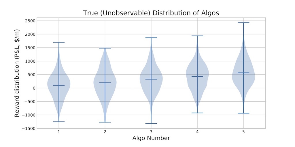
Figure 3. Algo Selection Problem: Distribution of Algo P&L
Also, in the name of simplicity, we assume that the Algo User’s only unknown is P&L. The volatility is known. This is a generally ok starting assumption as volatility can be approximated with a good precision (see Merton, 1980). Let’s assume annualized volatility of 10%. Then using a factor of 252*24*60 we obtain 10%/sqrt(252*24*60) as the volatility per minute (1.66 basis points/bps). Assuming average algo run of 30 minutes, that would translate to the volatility of 9 bps (1.66 times the square root of 30) in 30 minutes. And as we are interested in volatility of average price over the course of 30 minutes (rather than final price in the end of 30 minutes) we scale the number by the square root of 3 to obtain TWAP volatility of 5 bps or 500 $/m (exactly like in Figure 1).
The Algo User must have certain “beliefs” about the quality (meaning P&L distribution in a one-dimensional case) of the algos he is presented with. Those beliefs are shaped by the quality of the presentation material, reputation of the trading shop selling the algos or his personal relation with a salesperson offering the product.
All we want from those beliefs is that they should be flexible (not rigid like “Algo 5 is the best”). The most standard way to express belief is via Bayesian approach.
Figure 4 shows the basic illustration. The user believes (with a reasonably low degree of confidence) that the (unobservable) mean say P&L is 20, sees the realization of 10, builds a likelihood around observed value of 10 (orange bell curve) and arrive at the new estimate for mean around 15 (green bell curve).
This process allows him to update beliefs given the new evidence using Bayes formula which can be simplified to nothing more than a common sense equation like below:

In other words, the equation is nothing more than John Maynard Keynes famous “When the facts change, I change my mind. What do you do, sir?” statement. But it allows us to update our beliefs in mathematically consistent way (it is more complex than you would expect, see Kahneman, 2011 for examples).
The multi-arm bandit model we consider is called Bayesian bandits. The user starts with a set of beliefs which come from elsewhere (and in the case of user not willing to assume anything, the user can use “uninformative prior”) and follows a specific procedure (drawing from a prior) to select an algo. Then his beliefs are updated using standard formulas (see “conjugate priors” in simple case) and the procedure repeats as choose, observe and update-beliefs cycle. The procedure (called Thompson sampling, see Figure 2, right hand side) sounds like a naïve voodoo to a user not familiar with the literature but has been proven to perform remarkably well (see Honda and Takemura, 2014).
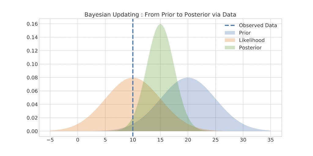
Figure 4. Prior, Data, Posterior Illustration
Financial Markets: Short Run Vs Long Run
One important caveat about theoretical literature on multi-arm bandits is that it concerns itself with asymptotic (or long run) results. But for most users in finance the long-run is irrelevant as the environment changes faster than they manage to accumulate statistical significance for long-run results (and asymptotically optimal methods may actually be sub-optimal short term).
Believing in long run in financial markets is a dangerous proposition. As the old adage goes: “there are old traders and bold traders, but no old, bold traders”
Therefore, we specifically focus on short run. We consider the first 100 algo runs and how they perform under different learning scenarios. Hundred runs is the round number and would broadly imply doing algo selection for 5 months every day (20 business days per month). This is quite a long period and most users would execute smaller amount of algos while the environment is still stationary.
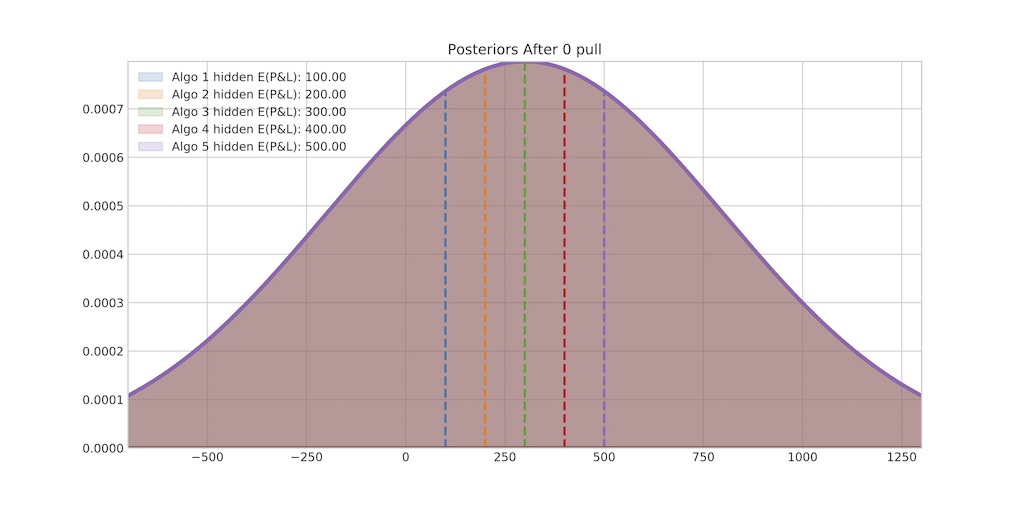
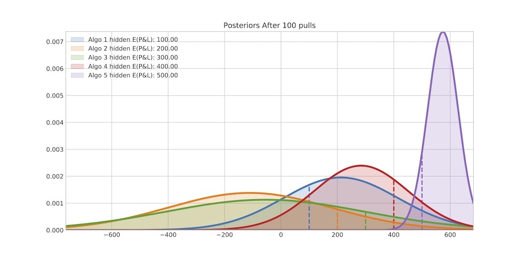
Figure 5. Learning About Underlying P&L, 0 pulls (Algo Runs) and 100 pulls (Algo Runs)
Simulation results
To formulate the problem again, we have an Algo User who has to select among 5 algos (with parameters as per Figure 1 and 3 where the expected P&L is not known). We assume that the user sees all those algos for the first time and does not have access to any historical P&L data. The user then assumes that all algos have the same mean (300 $/m, this might be algo average P&L across the industry) and assumes a very high uncertainty about this mean – volatility of the algo mean of 500 $/m (nothing to do with algo volatility). This is shown in Figure 5 (top chart). As one can see, all algos are the same to the user.
Then also the user starts to follow Thompson sampling procedure (see Figure 2, right chart and description above) by selecting one algo at the time, running it, recording the P&L and updating his beliefs about algo P&L as per the procedure. Figure 5 (bottom chart) shows the situation after 100 algo runs. The user still has large uncertainty about algo 1 and 2 because they have not been selected that often. Which is a good outcome given that we know (the Algo User does not) that their true P&L is 100 and 200 respectively, well below the optimal algo. Algos 3 and 4 have been chosen more frequently. Finally, algo 5 has been utilized most frequently and hence the curve (uncertainty) around this algo is the smallest. We can note that the user is overestimating the means of this algo (peak of the purple curve is over 500 which is the true expected P&L) but this will correct itself over the next runs.
How about the expected P&L of an algo selection strategy? Given the underlying expected Algo P&Ls (100, 200, 300, 400 and 500) it is clear that random selection strategy (also called “whoever I had lunch with last”) would yield an expected P&L of 300.
How do alternative strategies compare? The simulation results are given in Figure 6. I report cumulative P&L per algo run as it is most relevant (total P&L) while also the most easily interpretable number (for comparison with random strategy for example). For comparison, I also provide standard “average historical P&L” strategy performance – this strategy simply starts from some standard P&L estimate for each algo (e.g 0 but the initial condition does matter a lot!) and update average historical P&L for each algo. I call this “Argmax” strategy as python pandas function called Argmax selects the index of the maximum element (I do randomize the ties in simulation).

Figure 6. Algo Selection Strategy P&L
Panel A of Figure 6 shows that after a slow start the Bayesian strategy P&L improves markedly and reaches 475 $/m per algo run. As it is cumulative P&L (including the learning stage start from left hand side, algo runs from first runs) it is quite a high number. Argmax strategy on Panel A stumbles on what is called “local maximum” in optimization theory: it selects suboptimal algo with lucky run and sticks with it and other algos simply do not have a chance to show they are good. The starting value has a lot to do with it – starting from 0 takes a pessimistic view of the world. As a result, the expected P&L of this strategy when starting from 0 is only slightly above 300 (random selection).
Panel B shows the same Bayesian strategy but different Argmax strategy. All I change is that now the Argmax strategy starts from initial values of 300 $/m for each algo. This encourages more exploration at 300 $/m is more difficult to beat than $/m so bad algos (bad equilibria) are less likely to occur. A seemingly insignificant starting value selection results in a markedly different performance – it is now around 400 $/m per algo run, confidently beating the random strategy with the expected P&L of 300 $/m. Argmax strategy is what is typically used for algo selection as it is the easiest and most intuitive choice. Therefore, it is important to be aware of pitfalls
The initial under-performance of Bayesian versus Argmax strategy (Figure 5, Panel B) is a classical “explore versus exploit” trade-off. Bayesian strategy does exploit more and catches up with Argmax at around run 7 (blue line cross orange from below on Panel B)

Figure 7. Algo Information Aggregator
Pooling algo run information
The results in the previous section imply that after the initial learning state the algo learner figures out reasonably quickly which algos are worth running. Wouldn’t it be nice to have this information beforehand? If only Algo Users agree to share the information with each other! Of course, Algo Users would not want to share individual runs. That information can be very sensitive for their business. For example, they may have predicable buying and selling patterns and this information can be exploited by a front runner (e.g fellow Algo User) if made available. However, aggregates are far less sensitive. Figure 7 shows how this can be done.
Just to highlight the value of having someone else’s information (if there was any doubt) Figure 8 presents the result. If the first 100 runs are made available to Algo User in the form of Bayesian priors (set of means and standard deviations, see Figure 7) then the next 100 algo runs achieve almost perfect score. This is clearly an idealized view. In reality many things will contribute to less than perfect score even in case of information sharing:
- Algo Performance is not stationary; winners and losers change all the time.
- Algo performance is very state dependent – some algos are good in high volatility, some in a low volatility environment. Other market regimes (not just volatility) would be relevant as well.
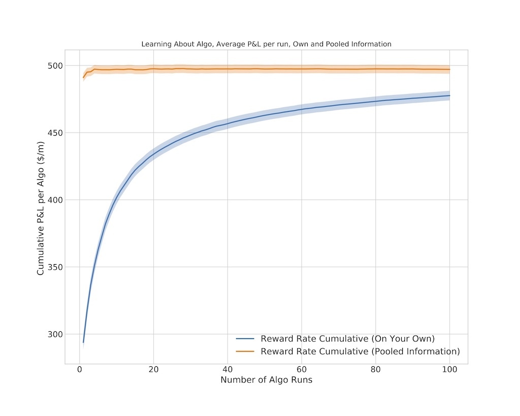
Figure 8. Simulation Result – Using Someone Else’s Info
Challenge for aggregation: Lots of bells and whistles
In a sense, the Algo User rents the algo vendor’s expertise in the following areas: trading (short term alpha), order placement, ECN connectivity and technology (OMS/EMS). Algo Providers design their algo offering with different levels of controls to make renting as flexible as possible:
- Algo type which is typically determined by a goal (normally referred to a benchmark which might lead to confusion). For example, implementation shortfall or arrival algo attempts to minimize slippage with respect to arrival price while TWAP algo attempts to minimize slippage to TWAP price. Both criteria can be penalized for volatility
- Algo urgency is a use parameter
- Liquidity selection – Algo User can manage the liquidity utilized by the algo.
Sometimes even algo type can be changed during the algo run. The above list suggest that the Algo User can rent what he wants from the algo vendor and leave the rest of the job for himself. Lots of Algo Users are professional traders who only rent the abilities of algo vendors to place orders, but manage execution urgency, and Limit Orders themselves.
Not surprisingly those bells and whistles create a lot of challenges for algo aggregation. One such example if shown on Figure 9. A user sets an aggressive limit price and the market goes down to fall below that limit price. It is the user, not the algo which is responsible for much of the P&L. But another user cannot reproduce this user’s skillset so would only be interested in the P&L portion attributed to the algo in the aggregated algo pool. This decomposition would have to be done by someone (user himself or better if some platform as the adjustments would have to be consistent across users).
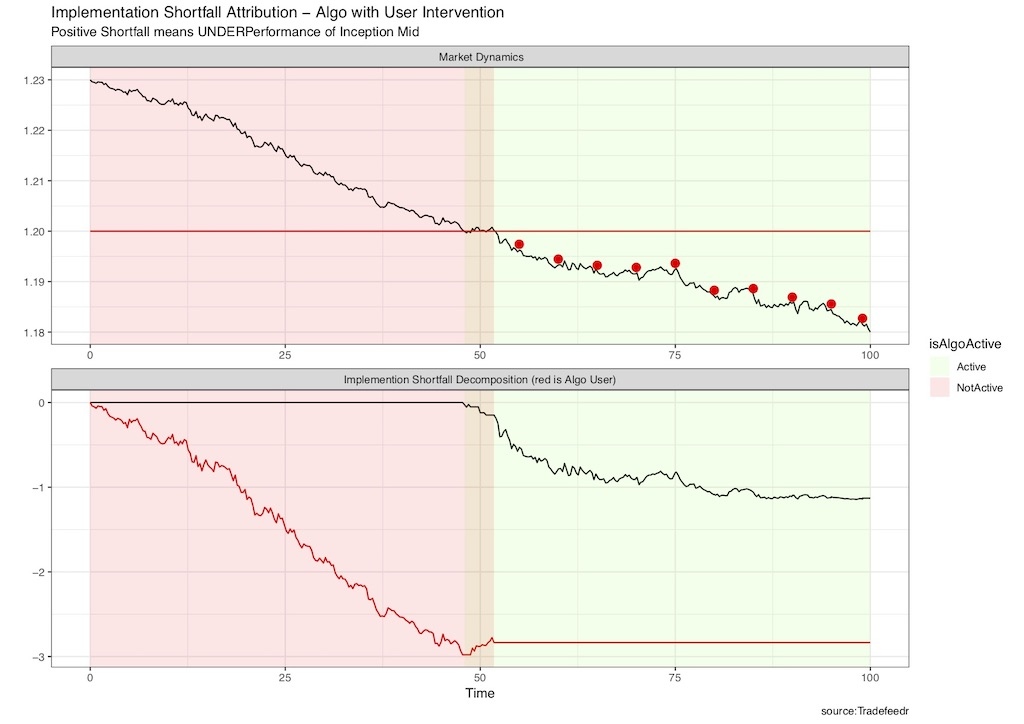
Figure 9. Algo Performance Decomposition. Buying a dog (algo) and barking yourself
Conclusions and Extensions
This article has barely scratched the surface of applying machine learning to algo selection. The emphasis is mainly on treating algos as a black box so the only way to learn about their performance is to run them (or obtain the run result of others, e.g. pooling). For this domain, multi-arm bandit setup maps almost perfectly.
Even in this domain lots of improvements are possible:
- Cross-algo and symbol learning. Of course, it only makes sense to directly compare algos with the same underlying. For example, a EURUSD algo should only be compared with EURUSD and preferably with the same characteristics. But what if you have lots of experience in EURUSD algos but want to expand this to GBPUSD. Surely, your first move should be towards you best EURUSD algo provider. This logic can be expressed scientifically via a contextual bandits algorithm. Two states are EURUSD and GBPUSD and the structure learns from both EURUSD and GBPUSD runs.
- Objective function. It is common knowledge that nobody likes risk. The setup presented maximized P&L assuming the risk is the same. It may not work in practice. For example, if P&L is the same you may prefer an algo that takes less market risk (or simply less time which is almost equivalent). Then, the mean(P&L)-variance objective function can be used as comparison as opposed to just the expected P&L as per example above.
References
Richard S. Sutton and Andrew G. Barto, 2018, Reinforcement Learning: An Introduction, Second Edition
Cameron Davidson-Pilon, “Bayesian Methods for Hackers: Probabilistic Programming and Bayesian Inference “, 2016, Addison-Wesley Data & Analytics
Merton, Robert, 1980, On estimating the expected return on the market: An exploratory investigation. Journal of Financial Economics, Volume 8, Issue 4, December 1980, Pages 323-361
Junya Honda and Akimichi Takemura, Optimality of Thompson Sampling for Gaussian Bandits Depends on Priors, Proceedings of Machine Learning Research, Volume 33: Artificial Intelligence and Statistics, 22-25 April 2014
Tze Leung Lai and Herbert Robbins. Asymptotically efficient adaptive allocation rules. Advances in applied mathematics, 6(1):4–22, 1985
Daniel Kahneman, 2011, Thinking, Fast and Slow, Penguin
Robert Skidelsky, 2005, John Maynard Keynes,
